I’ve just begun my second deep learning course with Prof Stanley Kok at NUS - for FT5011. Based on the first lecture alone, I have a feeling that this is going to be a great course. Stanley seems to be a very good explainer of concepts, and despite having learnt deep learning and neural networks before, there were still nuances from the first lecture that I want to write about.
How several linear graphs combine
Consider a shallow neural network with 3 nodes in its hidden layer. Mathematically, it can be represented as:
$$ y = f[x, \phi] \ = \phi_0 + \phi_1a[\theta_{10} + \theta_{11}x] + \phi_1a[\theta_{20} + \theta_{21}x] + \phi_1a[\theta_{30} + \theta_{31}x] $$
Each node is denoted as:
$$ \phi_1a[\theta_{10} + \theta_{11}x] $$
where $\phi_i$ is the ‘weight’ passed into each activation layer and the $\theta_j$ params are the coefficients of the linear functions themselves.
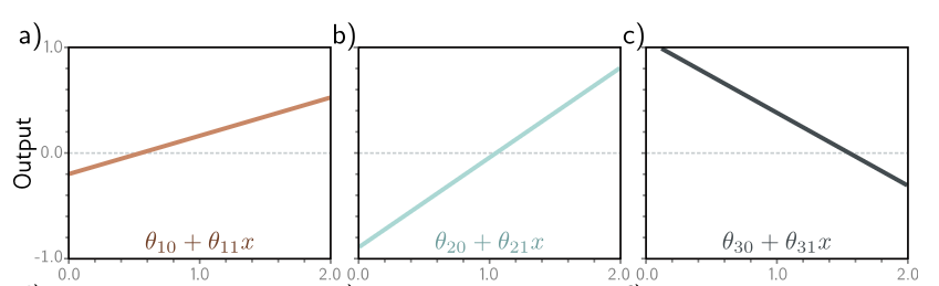
Consider the following linear function:
$$ \theta_{10} + \theta_{11}x $$
This maps to a straight line essentially. And the three lines in the shallow neural network eqn can be seen as three straight lines:
Now, of course, there’s some additional transformation on each of those lines, for instance, they’re fed into the activation function (which I’ll take as ReLU functions), before being multiplied by $\phi$.
The series of transformations can be visualized as such:
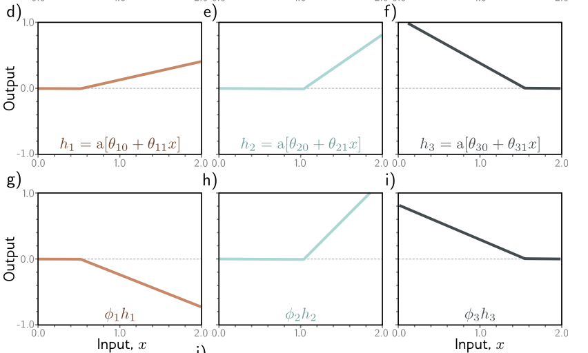
where the first row is the effects of applying a ReLU (negative outputs become flattened to 0), and the second row is transforming it with the $\phi$ value.
Now, at this step, how can we visualize these three lines combining in the shallow network function we shared above?
$$ y = f[x, \phi] \ = \phi_0 + \phi_1a[\theta_{10} + \theta_{11}x] + \phi_1a[\theta_{10} + \theta_{11}x] + \phi_1a[\theta_{10} + \theta_{11}x] $$
We literally add up each of those regions.
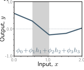
Let’s take the left most region for instance.
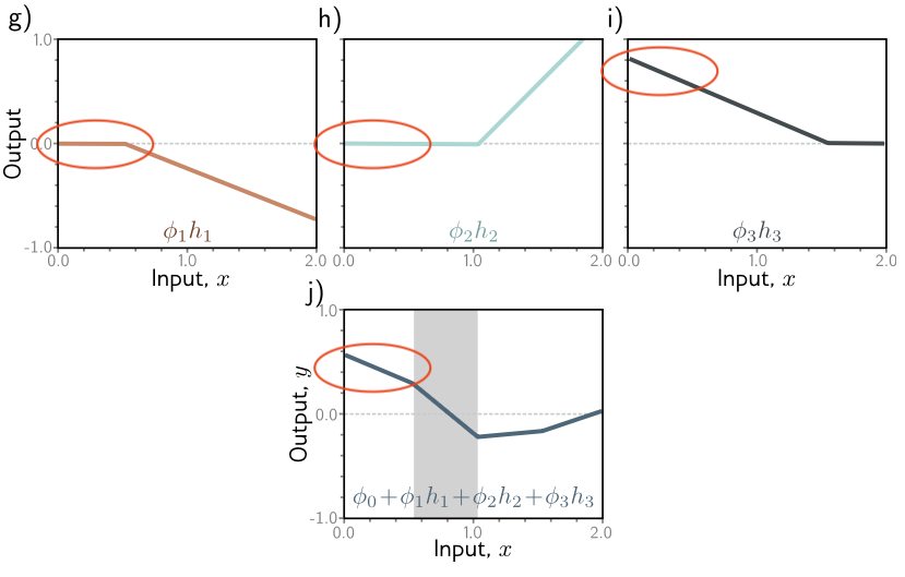
In graphs g) and h), we see that that region is essentially flat. Then, in i), we see a declining region. Combined together, we see a declining line as well in the final output.
Similarly, for the region on the right-
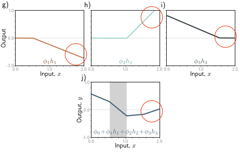
We see a declining region in g), a rising region in h), and a flat region in i). The combined effects is a slightly increasing region in the output.
The final output can still be represented graphically, and it maps to a curvy line!
There are three subtle but important points that I did not know prior to ‘seeing’ this relationship between the equations and the graphs.
- I didn’t know that a linear combination of three lines literally means adding the different regions of the graph together to form a final output line.
- That the mathematical representation actually maps to this kind of line combination process
- And that the number of ‘joints’ in the final output (3) corresponds to the number of ’nodes’, which in this case, refes to the number of linear lines.
Now, the corollary of point 3 is that the more the number of joints, or the more the number of ’nodes’ in your neural network, then the more ‘power’ your network has to create smoother contours and map arbitrarily curvy lines. That is also something that I did not know!
So if you need to have a function that actually predicts a wild shape, then you might need more ’nodes’ to give your model more ‘capacity’.
How multi-variate combinations look like on a plane
In the above example, we dealt with a single input x, fed into a network (or function) that has 10 parameters $\phi = {\phi_1, \phi_2, \phi_3, \phi_4, \theta_{10}, \theta_{11}, \theta_{20}, \theta_{21}, \theta_{30}, \theta_{31} }$.
However, there can also be cases where you have multiple inputs where $\textbf{x} = [x_1, x_2, … x_{D_i}]^T$, where $D_i$ is the number of dimensions of the inputs.
In this case, how can you visualize the combinations?
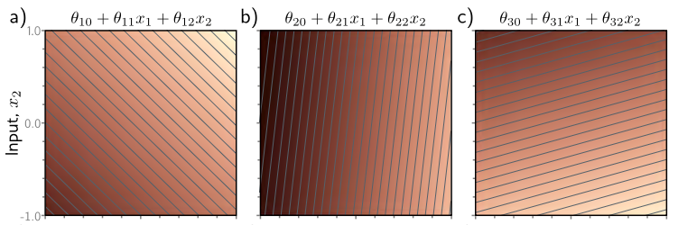
Similar to single-variate linear functions, we can visualize each of the linear functions separately.
$$\theta_{10} + \theta_{11}x_1 + \theta_{12}x_2 $$
In this equation, we see that $x_1$ is plotted on the x-axis, and $x_2$ value is plotted on the y-axis. The 2D plot is a contour plot, where the darker parts corresponds to smaller values and the lighter parts correspond to larger values. In the first diagram, we see that the outputs of the linear function can be represented in a contour plot of a particular direction and slope.
Because we’re dealing with a 2D input, the output will also be 2D - it’ll be a plane.
Now, each of those linear functions will produce a particular kind of plane, where each point on the plane represents a particular combination of $x_1, x_2$, and the output value is represented in colors.
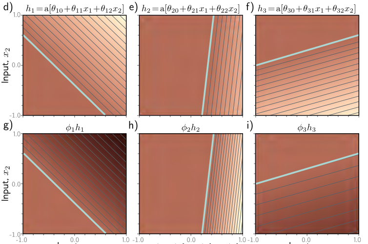
Similarly, we can apply transformations on the linear functions. In the first row above, we’ve applied a ReLU activation over the linear functions, rendering the negative values 0. For 0 values, we represent with flat colors. Then, we multiply the output with $\phi$, which has the effect of transforming the gradients of the planes.
Finally, by combining all of them, we get this:
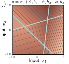
What is this? This is a polygon in 3D. Essentially, this is still a surface, but it’s a complex surface. It’s a surface where given each input combination, you may fall into different regions governed by the interactions between all those linear combinations.
On the notation when labeling your params in a neural network, in particular $\theta_{10}$
In the shallow neural network example, we see that although $\phi$ is labeled with a single integer, $\theta$ is labeled with an additional digit:
$$ y = f[x, \phi] \ = \phi_0 + \phi_1a[\theta_{10} + \theta_{11}x] + \phi_1a[\theta_{20} + \theta_{21}x] + \phi_1a[\theta_{30} + \theta_{31}x] $$
What is the significance of labeling $\theta_{10}$? What does 1 and 0 symbolize in this case?
It turns out that the shorthand for thinking about this is: this is the param to node 1 , from input 0.
$\theta_{10}$ - to node 1 from input 0
$\theta_{11}$ - to node 1 from input 1
$\theta_{20}$ - to node 2 from input 0
$\theta_{21}$ - to node 2 from input 1
The first number, then, represents the ’node number’, whereas the second digit represents, in some ways, the ‘input’ number. It’s a system where you designate the sender and receiver IDs.
The importance of being familiar with mathematical representation of models instead of visual representations
So being a visual learner (of sorts), I find that the visual representations of models often allow them to be fit into my mind. That is why I embarked in the past on projects such as visualizeML. However, the professor made an important point that made me ponder: he said that whilst understanding models visually is good for the start, as along as models become more complex, they may stop to serve you that well. And that is why it’s important to be familiar with mathematical notations because it’ll help us understand more complex models.
If true, I think this tip is a golden one.