The second class of FT5011 took us through loss functions. To be honest, my knowledge of loss functions is a little wonky. Like, I know the general idea, but beyond the simplistic model of “loss as sum of squared errors”, I really don’t know that much.
After being completely lost in the class, and subsequently reviewing the chapter on loss functions, I am happy to say that my mental model of loss functions has been sucessfully updated.
I’ll try to detail as much as possible the facts that I’ve learned.
1. The model as predicting a probability distribution instead of a point estimate of ‘y’ value.
This is by far the most groundbreaking thing that I’ve learned. Earlier, the way I understood ML/DL models is that they simply tell you what the answer is. For instance, a regression model will tell you the price given the output. A categorical model will tell you the class given the inputs (e.g. fish/cat). However, I realized that in practice, the model often spits out probabilities. For a regression problem, it spits out the probabilities that the output will be a particular predicted value. For a classification problem, it spits out the probability that the model will predict a certain class.
How on earth does the model spit out probabilities? To understand this, you’ll need to understand a little bit about probability distributions (I admit that my understanding of this has always been a little weak - and for the last 2 days, I’ve been brushing up on my basic probability theory, esp relating to conditional probability and probability distributions).
The crux of this mental shift is this: instead of having your model, $f[x, \phi]$, compute an output, you have it compute a probability distribution function $Pr(y|x)$ over possible outputs y given x. The simplest way to visualize this is with the bell curve (or gaussian distribution):
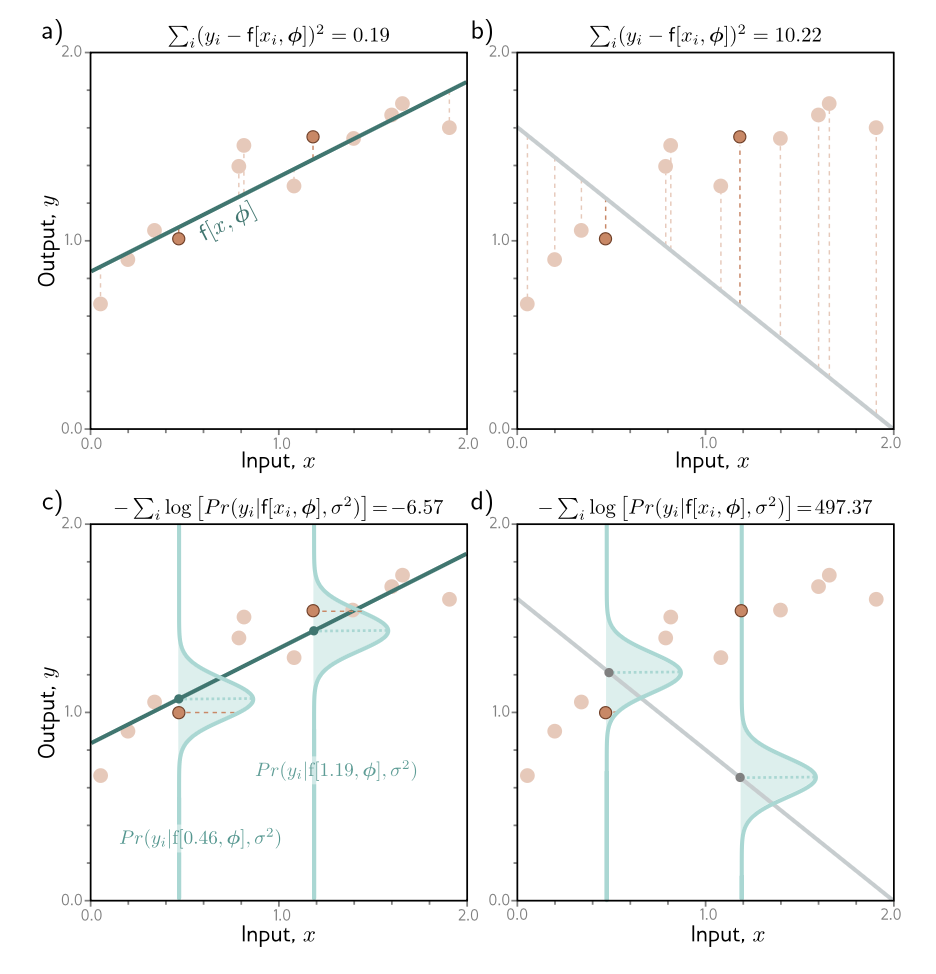
In a), we have your classic loss function, where the loss of the model is defined as a sum of squared loss of each point estimate. The output of your model is a regression line (essentially a mapping between y and x).
The new mental model can be seen in c), where our model outputs a unique gaussian distribution for each input of x. At x=0.446, for instance, our model outputs (or essentially constructs), a gaussian distribution with the equation: $Pr(y_i | f[0.46, \phi], \sigma^2)$ - a distribution with the mean at $f[0.46, \phi]$, and a variance at $\sigma^2$.
Now there’s quite a lot to unpack here. The standard conditional notation $Pr(y_i | f[0.46, \phi], \sigma^2)$ simply reads: the probability distribution of $y_i$ given those other 2 parameters, mean and standard deviation. The unspoken assumption here is that our model, formulated as such, essentially predicts the mean of this distribution (although there’s no reason to restrict our model to only predict the mean, as I’ll get to later).
What does this predicted distribution allow us to do? It allows us to say: okay, at x=0.46, there is a high probability that y value will be 1 (the mean); but other values of y is also possible, with varying degrees of probability. By factoring in probabilities, it allows our model to be a bit more robust.
More than that, the act of training essentially then reduces to: construct a probability distribution, such that the ground truth labels $y_i$ has the highest probability under our found distribution.
If our found distributions are like picture d) above, then it’s a poor model, or a model with high loss. If it’s like c), then it’s a model with low loss - a good model.
2. The accompanying formulas that this probabilistic view creates
In the previous chapters, our model was essentially outputs a fixed point estimate. Consider the formula for a shallow neural network:
$$ y = f[x, \phi] \ = \phi_0 + \phi_1a[\theta_{10} + \theta_{11}x] + \phi_1a[\theta_{20} + \theta_{21}x] + \phi_1a[\theta_{30} + \theta_{31}x] $$
Given x and $\phi$, this model will output a static singular y value.
Now, in order for us to have this model compute distributions instead, we first need find the right type of distribution we want to map to the problem (normal? bernoulli?), and then use the model to predict some aspect of the distribution parameters, $\theta$.
This is easier explained with a concrete example of trying to predict a single output like our shallow neural network model above (also known as univariate regression).
In this case, we first need a formula for the normal distribution that we want to ‘cast’ on each x value.
Now, the formula for the normal distribution is in fact this thing:
$\frac{1}{\sigma\sqrt{2\pi}} e^{-\frac{1}{2}(\frac{x-\mu}{\sigma})^2}$
So chatGPT probably has the best answer for why this equation is what it is. But basically, if you plot out this line in wolfram alpha (with mean=2 and var=0.5):
plot 1/sqrt(2*pi*0.5) * exp(-(y-2)^2/(2*0.5))
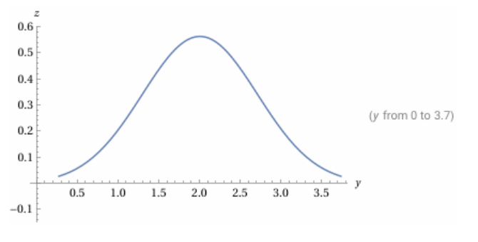 You’ll essentially see a normal equation where mean is at 2, and variance $\sigma^2$ is 0.5, making STD $\sigma$ 0.933.
The way ChatGPT answered it is, we simply want to build a function that’ll allow us to construct this shape, and has those properties.
Absolutely — let’s do this slow, intuitive, and motivation-first, no historical rabbit holes, no heavy measure theory. Think “why must it look like this?” rather than “how did Gauss do it?”. I’ll build it up in ideas → constraints → inevitable formula. What are we even trying to construct? We want a function
[
p(x)
]
that represents uncertainty around a typical value. Think: measurement noise, residuals, errors. 1. Constraint #1: “Errors don’t have a direction” Errors should be symmetric around the mean. If the true value is (\mu): So:
[
p(\mu + d) = p(\mu - d)
] This already kills lots of shapes. 👉 Conclusion: the distribution must depend only on distance from the mean, not direction. 2. Constraint #2: “Small errors are common, big errors are rare” This is crucial. As (|x - \mu|) increases: So we want: ** 3. Constraint #3: “Independent noise should add nicely”** This is the most important and least obvious part. Suppose: We want the shape of the distribution to remain the same
(just wider). That means: Adding independent noise should not change the family of the distribution This rules out almost everything. The only functions that survive convolution without changing shape are exponentials of quadratics. This is the deep reason Gaussians show up everywhere. 👉 This is the Central Limit intuition hiding underneath 4. Constraint #4: “Distance should matter quadratically” Why squared distance? Because: So we guess:
[
p(x) \propto e^{-k (x-\mu)^2}
] Not magic — just the simplest function that: At this point, the shape is fixed. 5. Why the exponential? Because probabilities multiply, but deviations add. If two independent deviations happen:
[
p(x_1, x_2) = p(x_1),p(x_2)
] Taking logs turns multiplication into addition:
[
\log p \propto - (x-\mu)^2
] Exponentiating brings us back to probability space. This is why: 6. Now the boring but necessary part: normalization So far we have:
[
p(x) = C \cdot e^{-k (x-\mu)^2}
] But probabilities must integrate to 1:
[
\int_{-\infty}^{\infty} p(x),dx = 1
] Solving that integral gives:
[
C = \frac{1}{\sqrt{2\pi\sigma^2}}
\quad \text{and} \quad
k = \frac{1}{2\sigma^2}
] That’s where the infamous (2\pi) comes from —
pure normalization, no modeling meaning. 7. Final result (nothing arbitrary left) \frac{1}{\sqrt{2\pi\sigma^2}}
\exp!\left(
-\frac{(x-\mu)^2}{2\sigma^2}
\right)
}
] Every term now has a job: 8. Why deep learning people care (even if they don’t derive it) This one equation explains why: If you assume:
[
y = f_\theta(x) + \varepsilon,
\quad \varepsilon \sim \mathcal{N}(0, \sigma^2)
] Then training a neural network by MSE is probabilistically optimal. 9. The one sentence takeaway The Gaussian isn’t special because it’s elegant —
it’s special because it’s the only distribution that survives symmetry, smoothness, and additive uncertainty. If you want next: Just tell me where you want to go 🚀ChatGPT explains the gaussian formula
[
\boxed{
p(x \mid \mu, \sigma^2)
Now the key thing here is to see that instead of predicting y, we want our model to predict $\mu$. The model’s formula therefore becomes:
$$Pr(y|f[x, \phi], \sigma^2) = \frac{1}{\sqrt{2\pi\sigma^2}}exp[-\frac{(y-f[x, \phi])^2}{2\sigma^2}]$$
Note, this then reads, the probability density function of y given this mean and SD is defined by this equation on the right, where $\mu$ is substituted for $f(x, \phi)$. Intuitively, our model outputs the mean, which then constructs a particular gaussian distribution.
This ultimately is the maximum likelihood criterion. The model computes a different distribution parameter $\theta_i = f[x_i, \phi]$; meaning, for each x, it gives rise to a different $\mu$. Each observed training output $y_i$ should have a high probability under its corresponding distribution $Pr(y_i|\theta_i)$. Our job therefore is to choose the model parameters so that they maximize the combined probability across all I training examples. Most directly, if we view the model as simply its final outputs and inputs, we have: $$\hat{\phi} = argmax_{\phi}[\prod_{i=1}^{I} Pr(y_i|x_i)]$$
Another view is to represent the intermediate params, $\theta$, which is a function of this distribution: $$ = argmax_{\phi}[\prod_{i=1}^{I} Pr(y_i|\theta_i)]$$
and if we want to make it even more explicit: $$= argmax_{\phi}[\prod_{i=1}^{I} Pr(y_i|f[x_i, \phi])]$$
These 3 conveys the same things.
3. The origins of negative log likelihood
It turns out that the formulas above are bad in practice because they are taking product of very small numbers. We tend to always reformulate the problem in terms of minimizing the negative log-likelihood:
$$\hat{\phi} = argmin{\phi}[-\sum_{i=1}^{I} log[Pr(y_i|x_i)]]$$
$$= argmin[L[\phi]]$$
And this, is essentially the final loss function a univariate regression problem.
In actual training, we are essentially minimizing this loss function:
$$L[\phi] = -\sum_{i=1}^{I} log[Pr(y_i|f[x_i, \phi], \mu^2)]$$
…where we’re substituting for the formula of the actual normal distribution:
$$L[\phi] = -\sum_{i=1}^{I} log[\frac{1}{\sqrt{2\pi\sigma^2}}exp[-\frac{(y-f[x, \phi])^2}{2\sigma^2}]] $$
4. Negative log likelihood equates to least squares
The surprising thing is that when we perform algebraic manipulation on the loss function, we end up with least squares function:
$$\hat{\phi} = argmin_{\phi} [-\sum_{i=1}^{I} log[\frac{1}{\sqrt{2\pi\sigma^2}}exp[-\frac{(y-f[x, \phi])^2}{2\sigma^2}]]] $$ …distributing the log… $$ = argmin_{\phi} [-\sum_{i=1}^{I} (log[\frac{1}{\sqrt{2\pi\sigma^2}}]-\frac{(y-f[x, \phi])^2}{2\sigma^2})]$$ …removing the first term as it doesn’t depend on $\phi$ (as we’re ultimately doing) differentiation
$$ = argmin_{\phi} [-\sum_{i=1}^{I} \frac{(y-f[x, \phi])^2}{2\sigma^2}]$$
…removing the denominator as it’s a scaling factor that doesn’t affect the position of the minimum…
$$ = argmin_{\phi} [\sum_{i=1}^{I} (y-f[x, \phi])^2]$$
And we get the least squared loss function!.
5. Doing inference in a probabilistic space
Given that our model no longer predicts y but predicts the mean, when we perform inference, we need to take the max of the predicted distribution:
$$\hat{y} = argmax_y[Pr(y|f[\textbf{x}, \hat{\phi}, \sigma^2])]$$
6. It’s entirely possible for your model to compute another parameter
In our running example, our model computes the mean of the distribution only. This means that every single point has a constant variance. This might not be realistic. We can construct a model such that $\sigma^2$ is also a learned parameter. The ideal parameters that minimize the loss becomes:
$$\hat{\phi}, \hat{\sigma}^2 = argmin_{\phi, \hat{\sigma}^2} [-\sum_{i=1}^{I} log[\frac{1}{\sqrt{2\pi\sigma^2}}exp[-\frac{(y-f[x, \phi])^2}{2\sigma^2}]]] $$
This essentially says that during training, we are finding both of these parameter such that loss (eqn on the right) is minimized.
Some jargon: when uncertainty of the model varies as a function of the input data, we call this heteroscedastic, as opposed to homoscedastic, where the uncertainty is constant.
The way to get both parameters is to train a neural network that computes both mean and variance, each as an output. We use the first output $f_1[x, \phi]$ to precict the mean, and the second output $f_2[x, \phi]$ to predict the variance.
However, given that the variance needs to be positive, we use a squaring function such that:
$\sigma^2 = f_2[x, \phi]$
Which results in the loss function:
$$\hat{\phi} = argmin_{\phi} [-\sum_{i=1}^{I} log[\frac{1}{\sqrt{2\pi(f_2[x, \phi])^2}}exp[-\frac{(y-f[x, \phi])^2}{2(f_2[x, \phi])^2}]]] $$
7. Binary classification
Whilst for univariate regression, we’re trying to predict a probability distribution in the shape of the gaussian one, for binary classification, the output space is a binary one, and hence, for every input, we’re trying to predict a Bernoulli distribution:
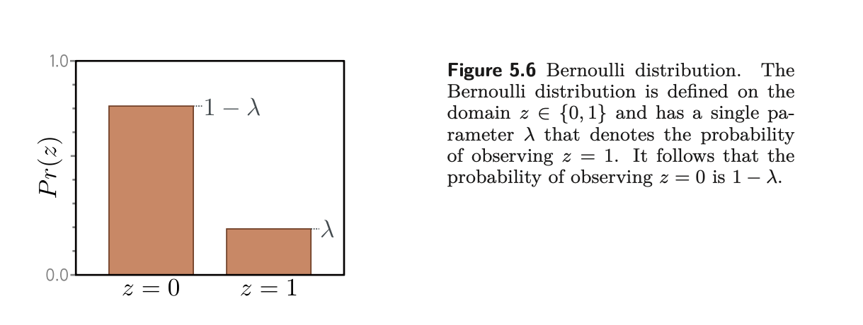
This is a distribution where your z represents only 2 outcomes.
There is only 1 parameter here, $\lambda$, and it represents the probability that y takes the value 1:
$$ Pr(y|\lambda) = \begin{cases} \lambda & y = 1 \ 1 - \lambda & y = 0 \end{cases} $$
This formula can also be written as:
$$ Pr(y|\lambda) = (1-\lambda)^{1-y} \cdot \lambda^y $$
In this case, our machine learning model $f[x, \phi]$ will predict a single parameter $\lambda$.
As this param must lie between 0 and 1, we apply sigmoid to the prediction, such that $\lambda$ = $sig(f(\textbf{x}, \phi))$
The probability distribution function thus becomes:
$$Pr(y|\textbf{x}) = (1-sig[f[\textbf{x}, \phi]])^{1-y} \cdot sig[f[\textbf{x}, \phi]])$$
Note that x and $\phi$ are in bold because they represent the vector.
…applying log and summing up the values across all training set…
$$L[\phi] = \sum_{i=1}^I -(1-y_i)log[1-sig[f[\textbf{x}, \phi]]] - y_ilog[sig[f[x_i, \phi]]]$$
This is known as the binary cross-entropy loss. This is also the expanded form of the following familiar form:
$$L = -(1-y)log(1-\hat{y}) - ylog(\hat{y})$$
The rule of thumb seems to be, once you ahve the probability distribution, you apply log over it, create a summation, and make it negative, to get your loss. Again, the theory is that once you have the distribution, you want to construct argmax across all training examples:
$$\hat{\phi} = argmax_{\phi}[\prod_{i=1}^{I} Pr(y_i|x_i)]$$
Such that you want the param to have the highest probability of matching ground truth.
This is translated to:
$$\hat{\phi} = argmin{\phi}[-\sum_{i=1}^{I} log[Pr(y_i|x_i)]]$$
Which after substitution becomes:
$$L[\phi] = -\sum_{i=1}^{I} log[Pr(y_i|f[x_i, \phi], \mu^2)]$$
and
$$L[\phi] = -\sum_{i=1}^{I} log[\frac{1}{\sqrt{2\pi\sigma^2}}exp[-\frac{(y-f[x, \phi])^2}{2\sigma^2}]] $$
Similarly, in binary classification, our Bernoulli distribution takes the form of:
$$Pr(y|\textbf{x}) = (1-sig[f[\textbf{x}, \phi]])^{1-y} \cdot sig[f[\textbf{x}, \phi]])$$
which after the negative log likelyhood trick, turns into the following loss function:
$$L[\phi] = \sum_{i=1}^I -(1-y_i)log[1-sig[f[\textbf{x}, \phi]]] - y_ilog[sig[f[x_i, \phi]]]$$
8. Multiclass classification
In this problem class, we might consider something like classifying digits - where given an input image, you output the probabilities of various categories.
In similar fashion, we first consider the prediction space y. $y \isin$ {1, 2, 3…K}. We thus choose a categorical distribution:
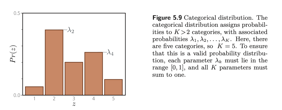
This has K parameters, $\lambda_1, \lambda_2…\lambda_K$ that determines the probability of each category.
There is one important constraint, which is that the sum of all $\lambda$ must equal to 1, and their values must be between 0 and 1.
Typically, we’ll use a network with K outputs to compute these K parameters. In order for the network to obey these constraints, we must pass the final K outputs into a softmax function.
$$softmax_k[z] = \frac{exp[z_k]}{\sum_{k’=1}^K exp[z_{k’}]}$$
This function has the following property: the exp part ensures positivity, and the sum in the denom ensures that the K numbers sum to 1.
The distribution is therefore:
$$Pr(y=k | x) = softmax_k[f[x, \phi]]$$
The negative log likelihood of the training data is therefore:
$$L[\phi] = -\sum_{i=1}^Ilog[softmax_{y_i}[f[x_i, \phi]]] \ = -\sum_{i=1}^I(f_{yi}[x_i, \phi] - log[-\sum_{k’}^Kexp[f_{k’}[x_i, \phi]]]) $$
Note on the expansion: you’re essentially substituting the softmax formula, which distributes the top and bottom over the log, the top cancels out, and you get $f_{y_i}[x, \phi]$ which is essentially the current categorical output of the model, minus the sum of all the categories (1 to k) to compress the total within 1.
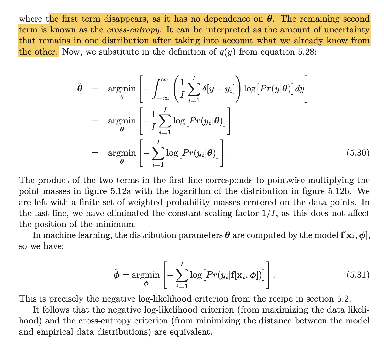
9. Cross entropy loss
The main thrust of the chapter is that by using negative log-likelihood, you will get the same results as cross-entropy loss. Cross-entropy, however, is derived in another fashion.
I won’t get into details here, but the gist is, you’re using KL divergence (which is a tool for finding how much one distribution differs from another) to minimize the model distribution $Pr(y|\theta)$ with the emporical distribution q(y). I am a little confused about the weighted sum of point masses part. But the results is the same. I’ll just attach the screenshots of the explanations here:
Also, here’s a good video explaining KL divergence:
And a subsequent video explaining cross-entropy loss:
9. Finally, the recipe for loss functions:
- Choose probability distribution over domain of predictions
ywith parameters $\theta$ - Set model $f[x, \phi]$ to predict one of these params, so θ= f[x,ϕ] and Pr(y|θ) = Pr(y|f[x,ϕ])
- To train the model, find the network parameters $\hat{\phi}$ that minimize the negative log-likelihood loss function over the taining dataset pairs:
$$\hat{\phi} = argmin{\phi}[-\sum_{i=1}^{I} log[Pr(y_i|x_i)]]$$
$$= argmin[L[\phi]]$$ 4. To perform inference, return either full distribution or the value where this distribution is maximized.
I think this chapter is really empowering because I’ve always treated loss functions as a bit of a black box, not really knowing why certain loss functions are used for certain problems, and also not knowing how to debug them should I need to. It’s crazy knowing that most loss functions can be constructed using such a ‘recipe’.