This is an overdue recap of the lecture I had 2 weeks ago, where we went through Stochastic gradient descent, momentum, and Adam.
I’ve learned the benefits of SGD before, so I won’t go that deeply into it. But I think what’s good about the lecture is how it anchors it in the mathematics.
Stochastic Gradient descent
To avoid being trapped in a local minimum, at each iteration, the SGD algorithm choose a random subset of training data and computes the gradients from these examples alone. This is known as a minibatch. The parameter update will then consider only that batch alone.
There are several good features of SGD:
- although it adds noise to the trajectory, it still improves the fit
- updates tend to be sensible, if not optimal
- because it draws training examples without replacement, it iterates through the dataset and all examples contribute equally
- less computationally expensive to compute gradient from a subset of data
- escapes the local minima in principle
- reduces chances of getting stuck near saddle points
Momentum
Now, this is where it gets more interesting. The idea of momentum is essentially that you don’t want each update to only be determined by the gradient change. You want it to be determined by the past gradient changes as well. In particular, you want it to be driven by the weighted sum of all the previous time periods, resulting in what is known as the momentum:
$$m_{t+1} = \beta \cdot m_t + (1-\beta) \sum_{i \isin \beta_t}\frac{\delta l_i[\phi_t]}{\delta \phi}$$
Now, $\beta$ is the term that controls how much the ‘past’ affects the overall gradient. $m_t$ refers to the previous momentum term (gradient encapsulated). Typically, you have $\beta$ values of around 0.9, which means that you want the past to hold 0.9 in terms of weight, whereas the current gradient of the loss only gets (1-$\beta$) which is 0.1.
If you expand out this equation, you can easily see that, at time step 3 for instance, the term comprises of information of the gradient at t2, t1, t0, etc. For instance:
$$m_3 = 0.9m_2 + 0.1d_2$$ $$m_3 = 0.9(0.9m1+0.1d_1) + 0.1d_1$$ $$m_3 = 0.9(0.9(0.9m_0 + 0.1d_0)+0.1d_1) + 0.1d_1$$
You can observe that $m_t$ is a recursive term that can be seen as a weighted sum of all the previous terms.
Adam
With this idea, we move on to Adam, an optimization algorithm that is probably the most used today. It combines the idea of momentum, with an additional adjustment that fixes the uneven update problem.
Uneven Update problem
Gradient descent with fixed step size makes large adjustments to parameters with large gradients, and small adjustments to params associated with small gradients. This is undesirable because the surface may be steeper in one direction than the other. Setting a larger learning rate will cause us to ‘overshoot’ the direction where a smaller update results in a larger change. In other words, the magnitude of gradient changes is different across directions - some might require smaller changes (steep surfaces), whereas others require aggressive changes (flatter surfaces).
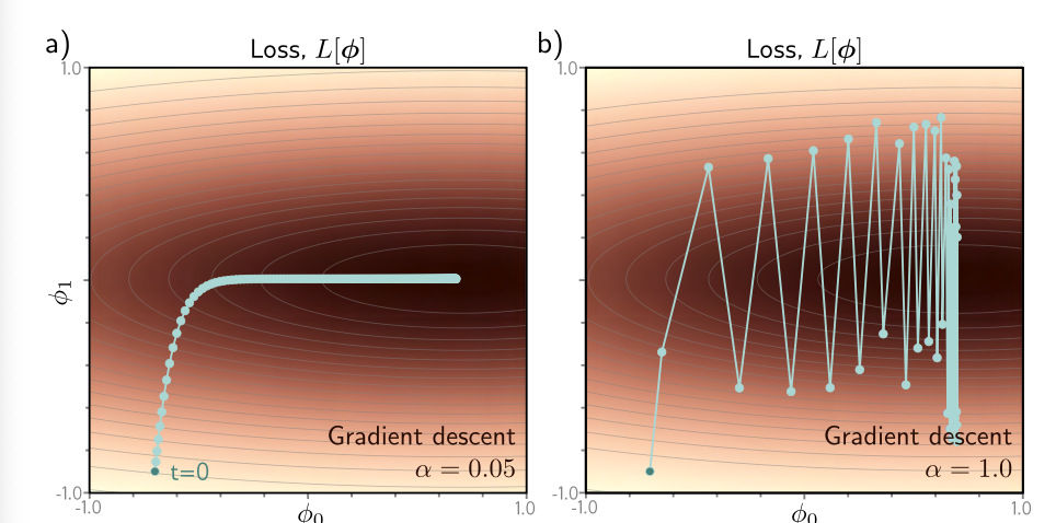
For instance, the surface in the graph below is uneven: the verticle direction descends quickly (steep), whereas the horizontal direction descends slowly (flatter). In the first diagram, a learning rate of 0.05 (which works for descending the steep surface), will cause the updates to be super slow once it reaches the flatter horizontal middle. If we try to increase the learning rate to 1, then we basically make huge leaps in the steep verticle surface, but as we move across the x-axis, the y-values fluctuate drastically.
The trick, then, is to normalize the gradients so that we move a fixed distance in each direction.
Here is the updates needed:
First, we just take the current gradient as the previous gradient: $$m_{t+1} = \frac{dL[\phi_t]}{d\phi}$$
Then, we square the loss to get rid of the sign: $$v_{t+1} = (\frac{dL[\phi_t]}{d\phi})^2$$
Finally, we update the params with the normalized second term: $$\phi_{t+1} = \phi_t - \alpha \cdot \frac{m_{t+1}}{\sqrt{v_{t+1}} + \epsilon}$$
So this operation $\frac{m_{t+1}}{\sqrt{v_{t+1}} + \epsilon}$ looks complex but is very very simple. Imagine $m_{t+1}$ is -5. $v_{t+1}$ will be $5^2$ and the denominator will simply be $\sqrt{5^2}$, which means the term divides by itself. ($\epsilon$ is just a very small number to make sure divisions by 0 doesn’t error out so we can ignore it.)
The result is that you get -5/5 which is -1. If your gradient is 100, you also get 100/100 which is 1. All you have left are 1 and -1 values - basically this operation reduces everything to 1 but preserves whatever original sign you have.
The full Adam
The full adam formula combines both the momentum idea as well as the normalization idea. This is the final formula:
$$\phi_{t+1} = \phi_t - \alpha \cdot \frac{\tilde{m_{t+1}}}{\sqrt{\tilde{v_{t+1}}} + \epsilon}$$
I’ll decompose some of the terms here slowly. So from this, we can see that the previous gradient $\tilde{m}{t+1}$ is divided by itself stripped of the sign ($\sqrt{\tilde{v}{t+1}}$), so this is normalization. However, you might have noticed that there are tilde signs on top of each ’m’ and ‘v’ . The reason is because we’ve modified the functions a little bit.
In the original conception of momentum, our $m_{t+1}$ term is like so:
$$m_{t+1} = \beta \cdot m_t + (1-\beta) \sum_{i \isin \beta_t}\frac{\delta l_i[\phi_t]}{\delta \phi}$$
This stays the same. We add a new $v_{t+1}$ term with a new parameter $\gamma$ that helps control the momentum of this term as well:
$$v_{t+1} = \gamma \cdot v_t + (1-\gamma) \sum_{i \isin \beta_t}(\frac{\delta l_i[\phi_t]}{\delta \phi})^2$$
This is essentially saying, how much of the previous iterations of itself do we want to consider as the denominator.
Now, we add this important but simple modification such that we don’t encounter the ‘cold start’ problem (where $m_0=0$ will result in a perpetually small $m_1$ update term):
$$\tilde{m_{t+1}}=\frac{m_{t+1}}{1-\beta^{t+1}}$$ $$\tilde{v_{t+1}} = \frac{v_{t+1}}{1-\gamma^{t+1}}$$
What this does is this. Consider a case where B = 0.9. At t=0, $m_t=0$ since there’s no previous gradient, so:
$$m_1 = \beta \cdot m_0 + (1-\beta) D $$ $$=0.9 \cdot 0 + (1-0.9) D $$ $$=0.1 D $$
…doing some bias correction…
$$\tilde{m_{t+1}} = \frac{\beta \cdot m_t + (1-\beta) \sum_{i \isin \beta_t}\frac{\delta l_i[\phi_t]}{\delta \phi}}{1-\beta^{t+1}}$$
$$\tilde{m_{1}} = \frac{\beta*0 + (1-\beta)D}{1-\beta^{0+1=1}} $$
$$= \frac{ \beta*0 }{ 1 - \beta} + \frac{(1 - \beta) D} {1-\beta}$$ $$= D$$
So essentially, all you’re keeping is the effects of the entire D term, and not its past!
Let’s work through an example of $m_2$:
$$m_2 = \beta \cdot m_1 + (1-\beta) D $$ $$=0.9 \cdot 0.1D + (1-0.9) D $$ $$=0.19 D $$
…doing some bias correction…
$$\tilde{m_{t+1}} = \frac{\beta \cdot m_t + (1-\beta) \sum_{i \isin \beta_t}\frac{\delta l_i[\phi_t]}{\delta \phi}}{1-\beta^{t+1}} $$
$$\tilde{m_{2}} = \frac{\beta*m_1 + (1-\beta)D}{1-\beta^{2}} $$
$$= \frac{ \beta*0.19D }{ 1 - \beta^{2}} + \frac{(1 - \beta) D} {1-\beta^{2}}$$
$$= \frac{ 0.9*0.19D }{ 1 - 0.81} + \frac{(1 - 0.9) D} {1-0.81}$$ $$= 0.473D + 0.526D $$ $$= 1.0000000000000002D$$
We observe a couple of things here. In the third line of the above math block, we see $\tilde{m_2}$ being decomposed into 2 terms. The first term is essentially the momentum term. The second term is the current gradient. We ultimately see the effects of this as favouring the second term slightly, whilst still retaining a significant chunk of the info from the first term.
As we iterate further down t, we will find that ultimately the first term will converge to 0.9 whilst the second term will converge to 0.1.
Okay I’ve spent way too long here, brain fried from my poor math.
But that’s about it! The fundamental idea of Adam is essentially an algorithm that helps us get out of cold start by favouring the current gradient heavily at the start; as well as combining elements where we normalize the gradient update to make it the same magnitude in all directions.