On the Math of Back Propagation

It’s incredible how entire models can be represented as a series of equations, and the entire process of back propogation (the spirit matter of deep learning) can also be represented as a series of equations. I’ll type this out fully when I have the time, but here’s what most neural networks are, abstracted:

The math of back propagation

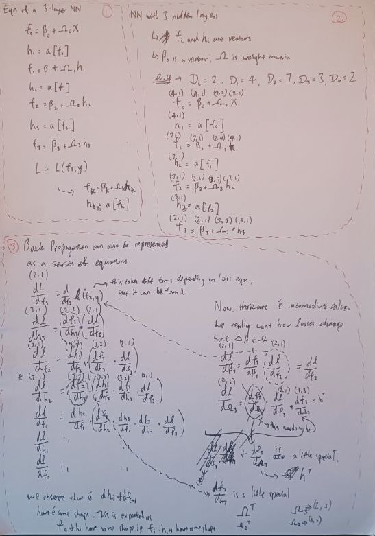
On the top left (1), you see a typical 3 layer neural network represented by a series of preactivations f and hidden units h functions. That’s all there is to it! It’s a very compact representation of a complex series of functional compositions.

On the top right, you see an actual walkthrough of the shapes of each function given certain model dimensions. I’ve chosen the classic 4-7-3 network with 2 inputs and 2 outputs.

Then, at the bottom, we note how backpropogation reduces to finding how dL varies with each individual layer’s $\beta$ and $\omega$, but to find that, we’ll need to find each layer’s dl/df and dl/dh. We see that the process of calculating up the tree from the final node $\frac{dL}{df_3}$ up to $\frac{dL}{df_0}$ is simply a question of applying chain rule.

One mental trick I’ve found for performing chain rule like this is ‘flip around’ the conventional way I do chain rule. For instance, typically to break down dl/df I’ll do: $\frac{dL}{dh}$ = $\frac{dL}{df}$ * $\frac{df}{dh}$. Now, I do $\frac{dL}{dh}$ = $\frac{df}{dh}$ * $\frac{dL}{df}$. The mental shortcut I use is to think about copying the bottom term first, and finding the ’next term’ in the chain (f comes after h if you refer to top equations), then times top term over ’next term’. Or another way to think about it is you’re building your chain upwards from dh. The benefits of arranging it like so is that you find that all the terms at the back (in brackets) are already computed - you only need to compute the first term! This makes back propagation a very efficient algorithm to finding derivatives of losses against all weights.

On some quirks of matrix calculus:

1. $\frac{dl}{d\Omega}$
The calculation of $\frac{dl}{d\Omega}$ (bottom right) results not in $\frac{dl}{df}*h$, but in $\frac{dl}{df}*h^T$. This is the reason:

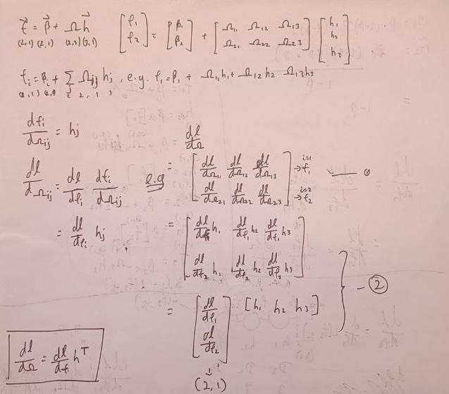
In short, by considering the Jacobin of $\frac{dl}{d\Omega}$, we realize that l needs to vary with each omega term, which means the shape needs to be the shape of omega essentially. Then, we substitute the chain rule composition into each omega derivative, and find that the result can be decomposed to a matrix multiplication of $\frac{dl}{df}*h^T$.

2. $\frac{df}{dh}$

The result of this is not omega, but $\Omega^T$. Take, for instance, the shape of $\Omega_3$ in our example: (2, 3). The resulting matrix multiplication when we reach the equation: $\frac{dL}{dh_3}$ = $\frac{df_3}{dh_3}$ * $\frac{dl}{df_3}$ sees $\frac{dl}{df_3}$ take the shape (2, 1) (since $f_3$ is of shape (2, 1)), which means that to properly multiply with this term, $\frac{df_3}{dh_3}$ needs to be of shape (3, 2), instead of (2, 3), which is the shape of omega. So this term essentially conforms to the needs of this matrix multiplication and we take $\Omega^T$.

So yes, these are just some of the quirks to consider when doing calculations on matrices, which might not be so obvious but is fundamental in getting the shapes of the gradients right. The key thing to remember is that when you’re differentiating losses over each of the params, the resulting shape always ends up being some kind of Jacobin because you need to calculate the perturbations between each individual parameter with the loss.

Alright I’ll get into more of the detailed math soon but for now I need to move on to the next chapter .