Parameter Initialization

Typically when initializing parameters ($\beta$, $\Omega$) for a network, we choose values from a standard normal distribution (with mean 0 and variance $\sigma^2$).

Now, the most important factor in preserving the stability of the network as we move past different layers (or functional transformations) is the variance of the initialization. This affects the magnitude of your preactivation f, activations h in the forward pass, as well as your gradients in your backward pass. This almost solely determines whether you’ll suffer from vanishing or exploding gradient problems.

Why variance?

Because in a standard normal distribution where the mean is at 0, a small variance essentially means small values of $\Omega$ given that data is clustered around 0, whereas a big variance means a big value of $\Omega$. This picture (albeit imperfect, kind of explains it):

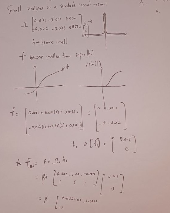
As you can see at the bottom, if the value of the weights are always 0.001, it shrinks the inputs h at an exponential scale. Similarly, if the values are larger, it’ll also increase very quickly.

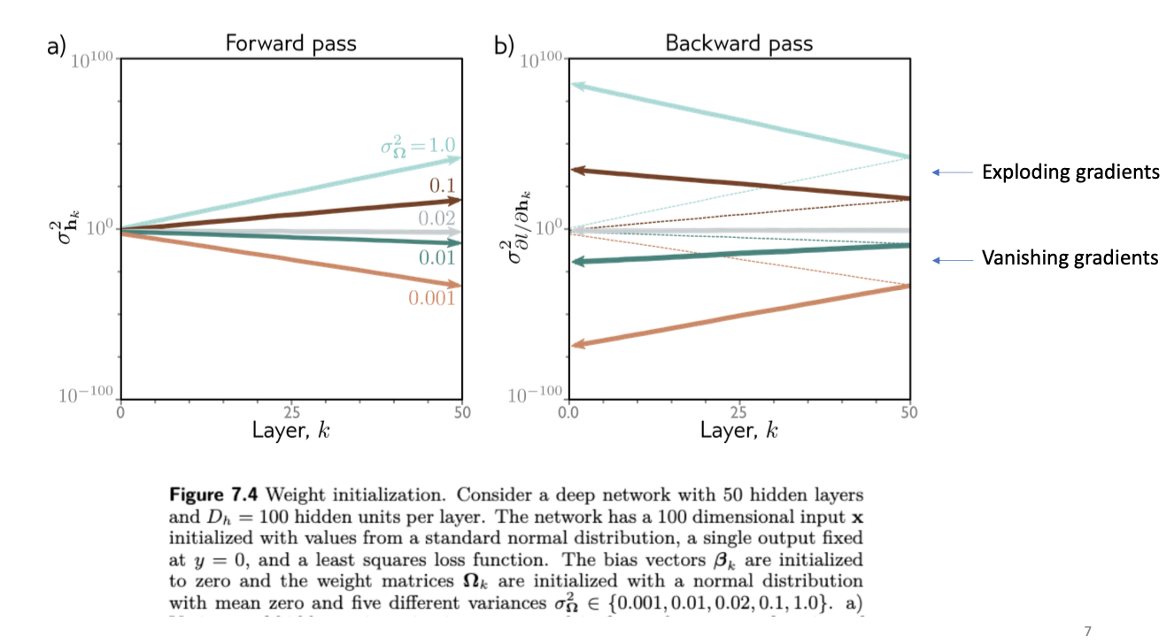
Key to this dynamic is that these numbers are constantly multiplying. So you need to choose ranges where these numbers, when multiplied together and added numerous times, are still within computable bounds. The following graph illustrates the dynamic:

One trick we can do to resolve this problem is called He initialization. Essentially, we want the variance of the hidden unit activations in the next layer to be the same as current layer. To do this, we set the variance of each layer as $2/D_h$. For instance, if a layer has 100 hidden units, and the previous layer has 50 hidden units, then the weights of the layer with 100 hidden units should be set to a variance of 2/50

(I understand that the statement above is not very precise, but I aim to capture a rough idea first).

Now, an interesting part is how do we derive the variance formula of $2/D_h$ in the first place.

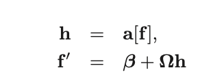
First, we consider two layers, h and f':

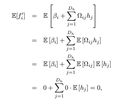
The expectation of f’ can be calculated as follows:

It follows that the variance of f’ is this:

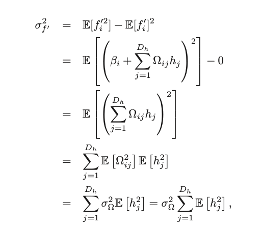
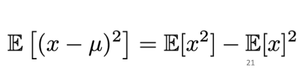
Now, on the first line, we leveraged this relationship in variances (if this is not clear to you, this can be easily worked out):

Given that twe know the second term is 0, now we need to find $f’^2$. Substituting the equation of f’, and doing some expectation manipulation, we get an expression in $h_j^2$.

Now, the challenge becomes finding an expression for the variance of f’ in terms of the variance in f.

The calculations are as follows:

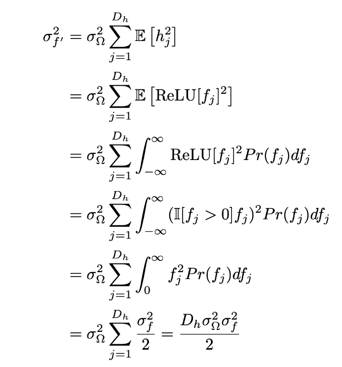
From line 1 to 2, we substituted the equation of h as a reLU function in f. Then, we substituted the formula for expectation of g(x), which is integral of g(x)*Pr(x).

Then, line 3 to 4, we know that ReLU can be represented as an indicator function, where as long as $f_j$ is positive, we keep; the rest we make to 0.

This also means that in line 5, we our integral for -ve sections of $f_j$ will just be 0, we “cancel out” the indicator function by just considering the positive valules of $f_j$.

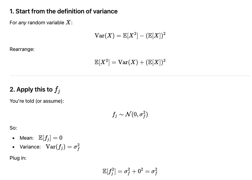
Finally, between line 5 and 6, we know that for a standard normal distribution, $E[f^2] = \sigma^2$. The reasoning is as below:

Which is why half of the equation of expection of $f^2$ (second last line) is equal to $\frac{\sigma_f^2}{2}$.

And finally, we get an equation of varaince of f’ with the variance of f!

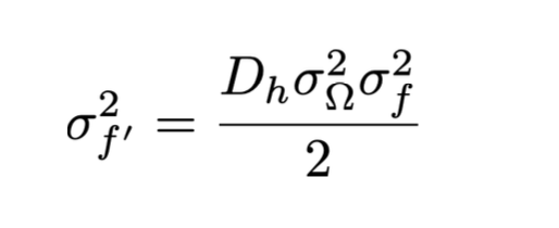
So if you want the ratio of $\sigma^2_{f’}$ to be the same as $\sigma^2_{f}$, then you equate $\frac{D_h\sigma_{\Omega}^2}{2} = 1$, and you get the relationship: $\sigma_{\Omega}^2 = \frac{2}{D_h}$

I think it’s a brilliant but non-obvious relationship in the weights to ensure that they don’t explode or disappear.