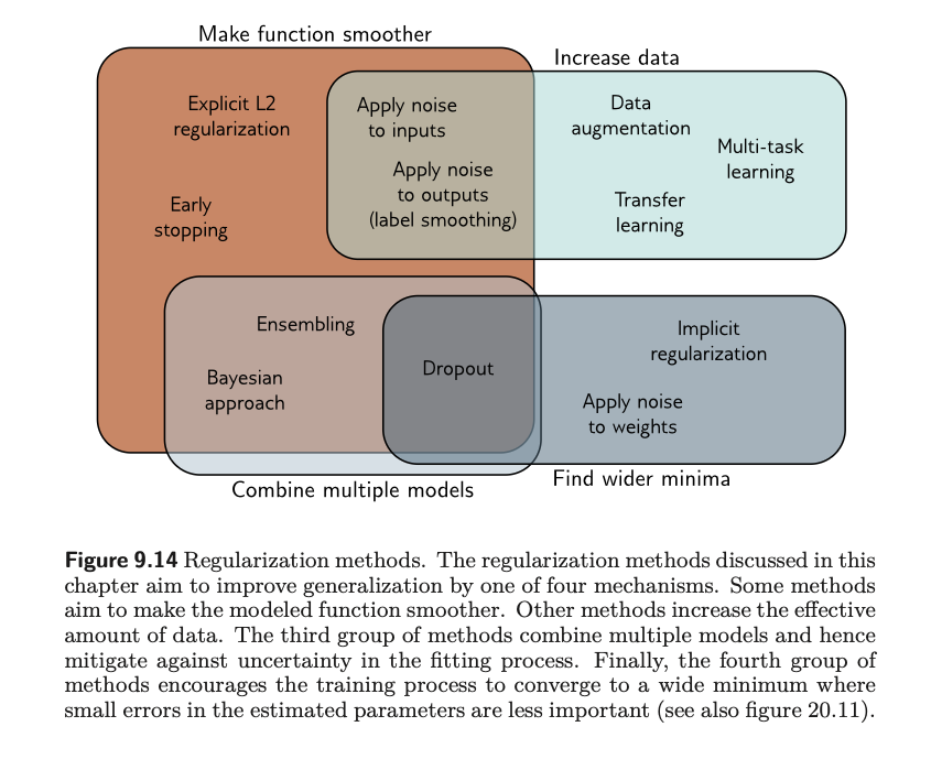
Regularization is the process of ‘smoothening out’ your loss function, such that it is less responsive to the peculiarities of a specific training dataset and therefore does better at interpolating to unseen data. It attempts to resolve the problem of fitting well on training data but doing badly on test data. This process involves adding a new term to the loss function. In machine learning, the term regularization is also generally used to refer to any strategy that helps improve generalization.
Specifically, regularization involves one simple tweak to your loss function:
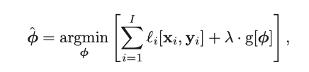
where $g[\phi]$ is a function that returns a scalar which takes larger values when the parameters are less preferred.
For instance, one of the most common regularization is the L2 regularization:
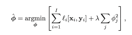
where j indexes the parameters. The second part of the term can be understood as sum of squared parameters, altered by a regularization factor $\lambda$. So if you think about it, the value of this loss function will be higher when the parameters of this model are big. Consider the following example:
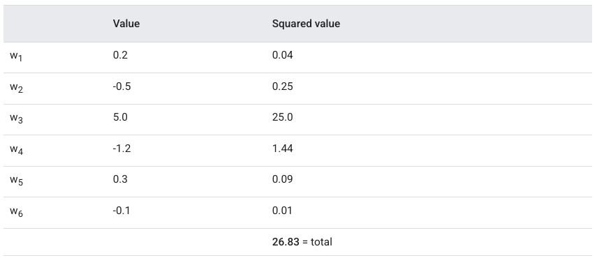
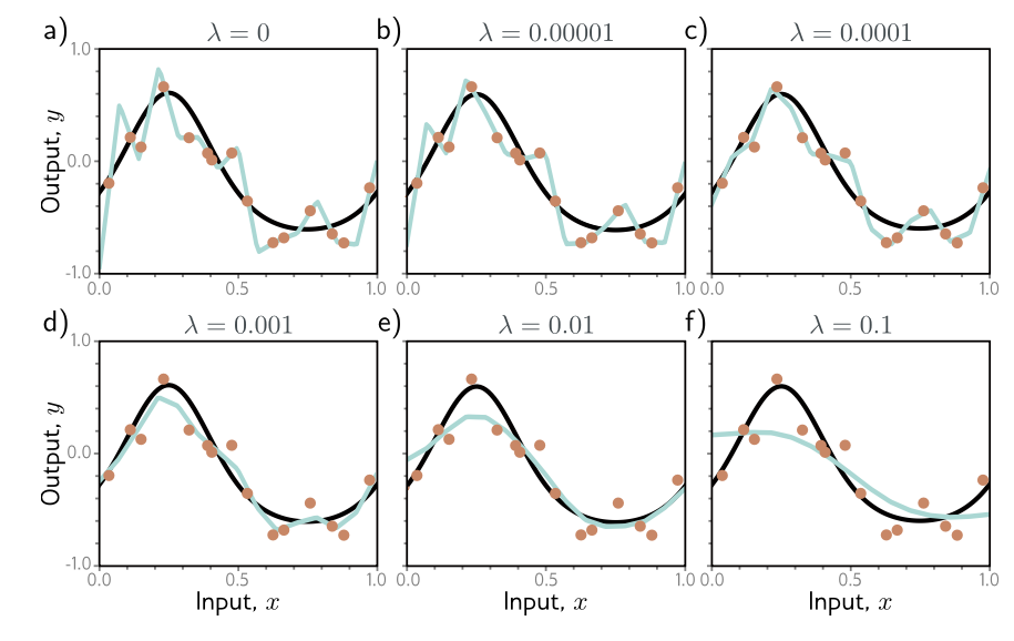
Notice that the weights close to 0 don’t affect the L2 regularization much, but larger weights do. By penalizing larger weights, we somehow ensure that the optimal model we get favours smaller weights. This is known as weight decay; and the overall effect is smoother output functions. Why? One way to see it is that if you set the $\lambda$ to be big, then the model is incentivized to set $\phi$ to be close to 0. Which means that for a lot of hidden units, their effects are minimal or even 0 - they’re deactivated. The result of that is a much simpler neural network - it loses expressivity.
Overall, regularization helps improve test performance for two reasons:
- If network is overfitting, it helps avoid slavish adherence to the data
- When network is over-parameterized, some extra model capacity describes areas with no trainign data. Here, the regularization term will favor functions that smoothly interpolate between nearby points, which is reasonable behavior in the absence of knowledge of the true function.
Implicit Regularization
I won’t get too much into details for this, but an interesting recent discovery is that gradient descent and stochastic descent don’t necessarily move neutrally to the minimum of a loss function - they both exhibit preference over some solutions over others. This is known as implicit regularization.
Heuristics to improve performance
If our goal is to improve generalizability of our model, then there are a few other tricks to consider.
- Early stopping
- stopping the training procedure before it’s fully converged
- reduce overfitting if model already captured coarse shape of the underlying function but has not yet had time to overfit to the noise
- one way to think about it is: since weights already initialized to small values, they simply don’t have time to become large; so early stopping has similar effect with L2 regularization
- another view: early stopping reduces effective model complexity, hence move back down the bias/variance trade-off curve
- Ensembling
- build several models and average their performance
- reliably improves test performance at the cost of training and storing multiple models and performing inference multiple times.
- How to train different models?
- use different random initializations
- use different dataset by re-sampling the training data with replacement and training a different model from each (known as bootstrap aggregating, or bagging)
- All create a smoother function.
- Dropout
- clamps a random subset (typically 50%) of hidden units to 0 at each iteration of SGD
- makes network less dependent on any given hidden unit and encourages weights to have smaller magnitudes so that change in the function due to the presence or absense of any specific hidden unit is reduced.
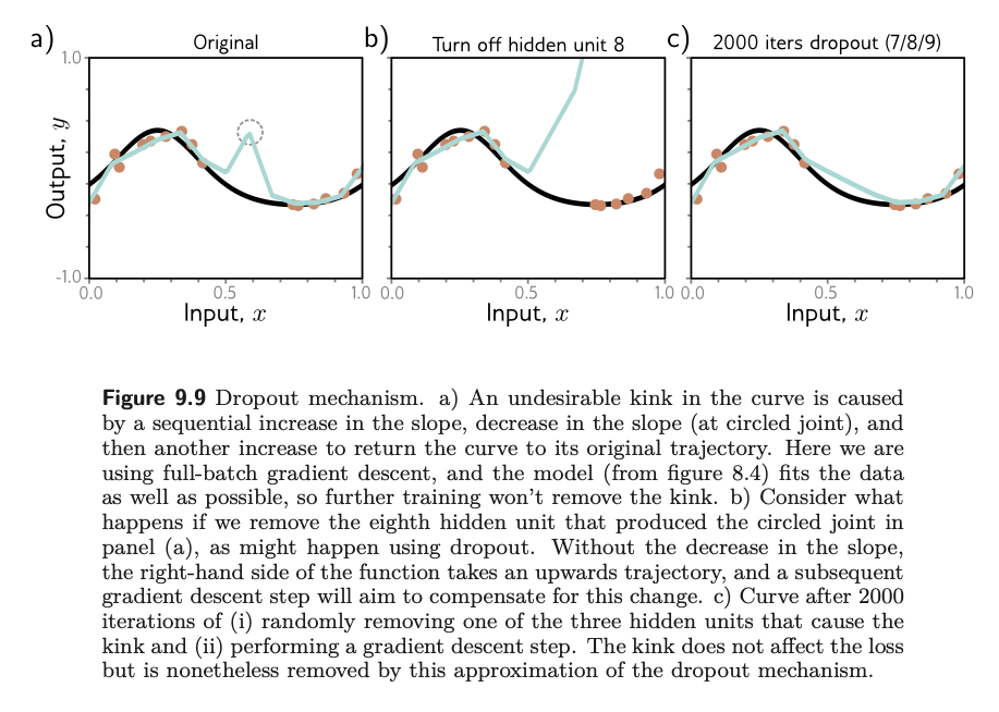
- has benefit of eliminating undesirable ‘kinks’ in the function that are far from the training data and don’t affect the loss.
- Adding noise
- dropouts can be interpreted as adding Bernoulli noise to network activations
- You can also add noise to other parts of the network during training to make final model more robust
- Option 1: Add noise to input data - > this smooths out the learned function.
- Option 2: Add noise to the weights -> encourages network to make sensible predictions even for small perturbations of the weights.
- Option 3: Purturb the labels
- MLE criterion aims to predict correct class with absolute certainty. The final activations (before softmax) are pushed to very large values for correct class and very small values for wrong classes
- we can discourage this overconfident behavior by assuming that proportion p pf training labels are incorrect and below with equal probability to other classes.
- Transfer learning
- Network pre-trained to perform a related secondary task for which data are more plentiful.
- Resulting model adapted to new task
- Typically done by removing last layer and adding one or more layers that produce a suitable output.
- Transfer learning can be viewed as initializing most of the parameters of the final network in a sensible part of the space that is likely to produce good solutions.
- Self-supervised learning
- Everything above assumes we have a lot of data for secondary task. If not, we can create large amounts of ‘free’ labeled data using self-supervised learning. Two types: generative and Contrastive
- Generative self-supervised learning: part of each data example is masked, and secondary task is to predict missing part.
- Contrastive: paris of examples with commonalities are compared to unrelated pairs. E.g. for images a secondary task might be to identify whether pair of images are transformed versions of one another or are unconnected.
- Dataset augmentation
- flip/distort, rotate, blur the dataset.
- audio: amplify or attenuate different frequency bands
In summary: