When we’re training our models, we’re minimizing loss. Yet, not all loss are created equal. Broadly speaking, there are 3 sources of errors:
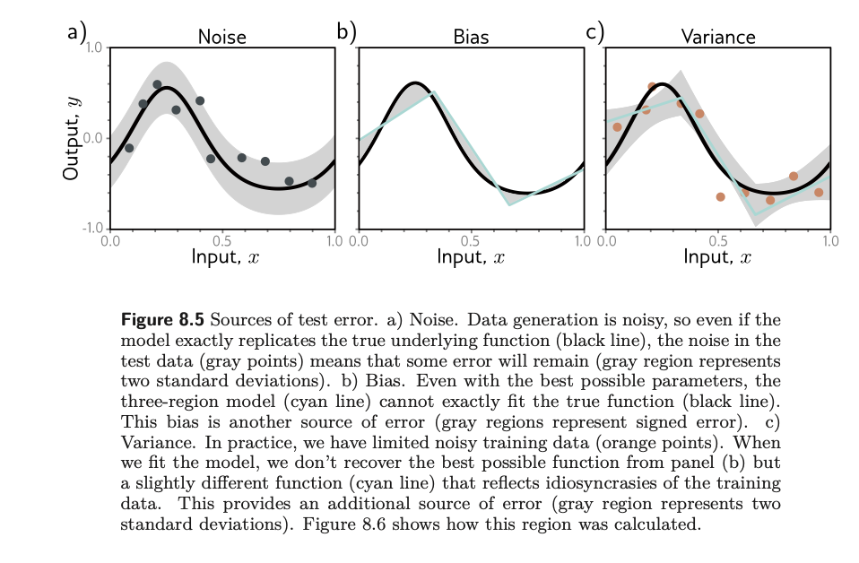
Noise
Noise is the inherent randomness of the test data. Assuming that you have a model that perfectly fits the true underlying function, the test data you draw will still lie within the SD of the true data. This is error that cannot be gotten rid of.
Bias
Bias refers to the implicit ‘bias’ of your model, or the shape of your model. If your model is not flexible enough, it can never fit a complex shape.
Variance
In practice, every time we train a model, we’re taking a draw at the training dataset. Every draw will be somewhat different. We end up having a slightly different function each time that reflects the idiosyncracies of the training dataset.
The interesting thing is that it’s also possible for us to find a mathematical explanation and definition of these three sources of errors.
Mathematical basis of noise, bias, variance
Consider a 1D regression problem:
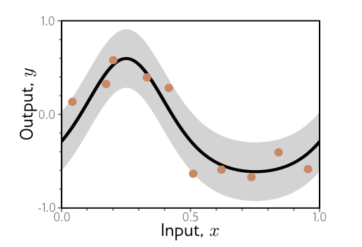
The data generated has additive noise with variance $\sigma^2$, and we can observe different output y for the same input x, so for each x, there’s a distribution where expected value of y follows:
$E_y[y[x]]$ = $\int y[x]Pr(y|x),dy = \mu[x]$
This is just an expectation in y[x]. And that’s the formula for expected value of f(x). Note: the $\mu[x]$ just means, if you pass in a fixed x, what is the mean of the distribution (imagine the vertical gaussian distributions) - that’s your expectation in y.
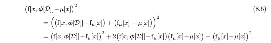
Now, consider the loss function. With a bit of manipulation, we get it to this form:
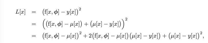
In the second step, all we did was a benign subtracting and adding of a $\mu[x]$ term, which does nothing. Then we apply the square.
We now calculate the expected loss $E_y[L[x]]$, which can be thought of as: the average loss I would get if I could observe all possible y[x] values generated by the data distribution.
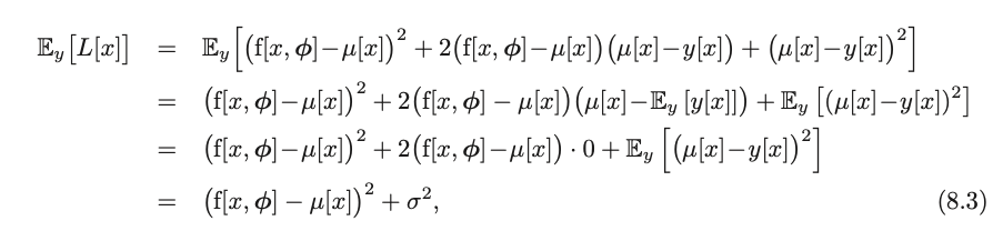
This idea requires a bit of unpacking. I have a loss function, yes. Now, this loss function is stochastic - which means that, given an input x, it’s not certain that I would generate a deterministic output y. Given that loss is a function of y[x] (which can be interpreted as draws of ground truth), loss itself is random. Think of it as, if I draw a y that lands higher, my loss will be higher. Thus, it’s also entirely possible to conceptualize a mean of loss, which asks: “if I repeatedly sample the world at input x, what loss do I expect to get on average?”.
And in the workings, given that x is fixed, and phi is fixed, the only source of randomness will be in y, so we take expectation only on the y terms. And in line 2, we see that the term $\mu[x] - E_y[y[x]]$ is actually equal to 0 given that by definition, $E_y[y[x]]$ is $\mu[x]$ as explained earlier (imagine gaussian).
Which breaks it down to 2 sources of error: the first term is the squared deviation of the model output with the true function mean, and the second term is the noise.
Now, this first term:
$$(f[x, \phi] - \mu[x])^2$$
can be further broken down into bias and variance.
$\phi$ depends on the training dataset $D={x_i, y_i}$, so more accurately, our f should be written as $f[x, \phi[D]]$. The training dataset is a random sample from a data generation process, so with different sample of training data, we would learn different parameter values. The expected model output $f_\mu[x]$ with respect to all possible datasets D is thus:
$$f_\mu[x] = E_D[f[x, \phi[D]]$$
This just means, after taking multiple training datasets, what is the expected model output? The function is thus $E_D$ to denote that dataset is the random variable here.
Returning to our first term: $$(f[x, \phi] - \mu[x])^2$$
When considering the draw of the dataset, we substitute $\phi$ with $D[\phi]$, and then do that same trick where we add and subtract the expected model output wrt all possible datasets:
Then, we take the expectation with respect to dataset D on both sides:

The middle term gets reduced to 0 in a similar step above, and the third term doesn’t depend on $E_D$ so we take it out of the expectation. We now have an expression in $E_D$.
Now, remember our expectation of the loss was:
Taking the ’effects’ of random Dataset into the picture, we take $E_D$ on both sides, and we get:
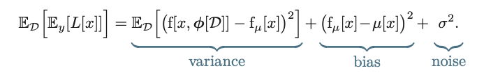
Now all these is a needlessly complicated (but theoretically sound) way of saying that, the ultimate errors in your data is dependent on these three things.
This is known as bias-variance decomposition.
Practical aspects: Reducing Variance
Now, given that we know that variance is is a result of limited noisy training data, it follows that we can reduce variance by taking more draws of the training data. This averages out the inherent noise and ensures that the input space is well sampled. In practice, this means that adding training data almost always improves test performance.
Practical aspects: Reducing bias
If the bias is the inability of the model itself to map onto the underlying function, then we just need to create better models to get better mapping.
Practical aspects: Bias-variance trade-off
There are cases where when you increase model capacity (reducing bias), you get more variance. This phenomenon can be illustrated as follows: imagine you have a robust model that have 50 joints. It can really track every single y value. What this also means is that a lot of the inherent variance you get when you draw different samples of the dataset is being tracked. This results in the model not being able to generalize well, and overfitting occurs. In this case, you sacrificed variance for lower bias (better model).
Double Descent
There was a recent phenomenon discovered which is that in many datasets, after completely overfitting the data and having the test results suffer, increasing the number of layers will then again cause test errors to drop.
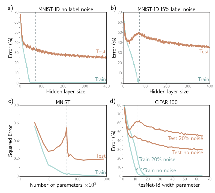
In the first image, we see an MNIST-1D training with no label noise. If there’s no label noise, that means that x will deterministically map to y. This also means that the only sources of error in the dataset is variance as well as bias. Variance being: variation between each draw of the dataset; and bias being how well our model can represent the underlying data.
As we can see, as our model increasingly lowers bias by adding more layers, test results are always going down. There is no overfitting - why? Because without noise, every training point lies exactly on the true function. Any model that interpolates the training data is also interpolating the true function $\mu(x)$. So increase in memorization doesn’t mean harm to test results.
Model variance still exists, as different datasets still give differently fitted models. But as training data increases, their predictions converge to $\mu(x)$ as all models that fit the data are fitting the same function.
Now, if we add label noise to the mix (which is most representative of real world data), we see that as the model capacity increases, there reaches a point where we are just modeling the noise or variance in the training data, and we fail to generalize to test data. It’s only after a massive increase in hidden layer size, that we can begin to generalize well again.
One theory of why that happens is that as we add more capacity to the model, it interpolates between the nearest data points in a high dimensional space increasingly smoothly.
To understand why performance continues to improve as we add more parameters, note that once the model has enough capacity to drive the training loss to near zero, the model fits the training data almost perfectly. This implies that further capacity cannot help the model fit the training data any better; any change must occur between the training points. The tendency of a model to prioritize one solution over another between data points is known as its inductive bias. The model’s behavior between data points is critical because, in high-dimensional space, the training data are extremely sparse. The MNIST-1D dataset has 40 dimensions, and we trained with 10,000 examples. If this seems like plenty of data, consider what would happen if we quantized each input dimension into 10 bins. There would be 1040 bins in total, constrained by only 104 examples. Even with this coarse quantization, there will only be one data point in every 1036 bins! The tendency of the volume of high-dimensional space to overwhelm the number of training points is termed the curse of dimensionality.
I don’t fully get this, but it’s also not very important for me to get this at this point.
But that’s about it! It’s good to be able to decompose error into its various forms, given that a large part of what we’re doing is to minimize those exact errors.